|
8.3
general documentation
|


|
|
8.3
general documentation
|
|
In code_saturne, a SLES means a S parse L inear E quation S olver. When using CDO/HHO schemes, the settings related to a SLES is stored in the structure cs_param_sles_t
To access more advanced settings, it is possible to retrieve this structure when one has a pointer to a cs_equation_param_t Simply write:
To get a full access to the low-level structures handling the linear algebra in code_saturne, please consider to edit the function cs_user_linear_solvers For a Finite Volume scheme, this is the main way to proceed.
Several examples are detailed hereafter to modify the default settings related to a linear solver.
For a symmetric positive definite (SPD) system, the solver of choice is the conjugate gradient (CS_PARAM_SOLVER_CG) or its flexible variant (CS_PARAM_SOLVER_FCG). In this case, a good preconditioner is a multilevel algorithm such as an algebraic multigrid (AMG). Different multigrid techniques are available when using code_saturne depending on the installation configuration (in-house implementations or algorithms available from PETSc and/or HYPRE libraries). Please refer to this section, for more details about AMG techniques.
Here is a second example:
If the external library PETSc is available, one uses its algebraic multigrid, otherwise one uses the in-house solver. Here a flexible conjugate gradient (fcg) with a diagonal preconditionning (jacobi).
By default, in-house solvers are considered. With some choices of solver or preconditioner, one has to use an external library. The external libraries which can be linked to code_saturne are:
CS_EQKEY_SOLVER_FAMILY allows one to specify the family of linear solvers to consider. This can be useful if an automatic switch is not done or when there are several possibilities. For instance,
Available linear solvers are listed in cs_param_solver_type_t and can be set using the key CS_EQKEY_SOLVER and the key values gathered in the following table:
| key value | description | associated type | available family |
|---|---|---|---|
"amg" | Algebraic MultiGrid (AMG) iterative solver. This is a good choice to achieve a scalable solver related to symmetric positive definite system when used with the default settings. Usually, a better choice is to use it as a preconditioner of a Krylov solver (for instance a conjugate gradient). For convection-dominated systems, one needs to adapt the smoothers, the coarsening algorithm or the coarse solver. | CS_PARAM_SOLVER_AMG | saturne, PETSc, HYPRE |
"bicgs", "bicgstab" | stabilized BiCG algorithm (for non-symmetric linear systems). It may lead to breakdown. | CS_PARAM_SOLVER_BICGS | saturne, PETSc |
"bicgstab2" | variant of the stabilized BiCG algorithm (for non-symmetric linear systems). It may lead to breakdown. It should be more robust than the BiCGstab algorithm | CS_PARAM_SOLVER_BICGS2 | saturne, PETSc |
"cg" | Conjuguate gradient algorithm for symmetric positive definite (SPD) linear systems | CS_PARAM_SOLVER_CG | saturne, PETSc, HYPRE |
"cr3" | 3-layer conjuguate residual algorithm for non-symmetric linear systems | CS_PARAM_SOLVER_CR3 | saturne |
"fcg" | Flexible version of the conjuguate gradient algorithm. This is useful when the preconditioner changes between two successive iterations | CS_PARAM_SOLVER_FCG | saturne, PETSc |
"fgmres" | Flexible Generalized Minimal Residual: robust and flexible iterative solver. More efficient solver can be found on easy-to-solve systems. Additional settings related to the number of directions stored before restarting the algorithm (cf. the key CS_EQKEY_SOLVER_RESTART) | CS_PARAM_SOLVER_FGMRES | PETSc |
"gauss_seidel", "gs" | Gauss-Seidel algorithm (Jacobi on interfaces between MPI ranks in case of parallel computing). No preconditioner. | CS_PARAM_SOLVER_GAUSS_SEIDEL | saturne, PETSc, HYPRE |
"gcr" | Generalized Conjugate Residual: robust and flexible iterative solver. More efficient solver can be found on easy-to-solve systems. This is close to a FGMRES algorithm. Additional settings related to the number of directions stored before restarting the algorithm (cf. the key CS_EQKEY_SOLVER_RESTART). This is the default solver for a user-defined equation. | CS_PARAM_SOLVER_GCR | saturne, PETSc |
"gmres" | Generalized Conjugate Residual: robust iterative solver. More efficient solver can be found on easy-to-solve systems. Additional settings related to the number of directions stored before restarting the algorithm (cf. the key CS_EQKEY_SOLVER_RESTART) | CS_PARAM_SOLVER_GMRES | saturne, PETSc, HYPRE |
"jacobi", "diag", "diagonal" | Jacobi algorithm = reciprocal of the diagonal values (simplest iterative solver). This is an efficient solver if the linear system is dominated by the diagonal. No preconditioner. | CS_PARAM_SOLVER_JACOBI | saturne, PETSc, HYPRE |
"mumps" | sparse direct solver from the MUMPS library (cf. [1]). This is the most robust solver but it may require a huge memory (especially for 3D problems). By default, it performs a LU factorization on general matrices using double precision. More options are available using the function cs_param_sles_mumps and the function cs_param_sles_mumps_advanced. More options are available through the user-defined function cs_user_sles_mumps_hook | CS_PARAM_SOLVER_MUMPS | mumps, PETSc (according to the configuration) |
"sym_gauss_seidel", "sgs" | Symmetric Gauss-Seidel algorithm. Jacobi on interfaces between MPI ranks in case of parallel computing). No preconditioner. | CS_PARAM_SOLVER_SYM_GAUSS_SEIDEL | saturne, PETSc |
"user" | User-defined iterative solver (rely on the function cs_user_sles_it_solver) | CS_PARAM_SOLVER_USER_DEFINED | saturne |
Available preconditioners are listed in cs_param_precond_type_t and can be set using the key CS_EQKEY_PRECOND and the key values gathered in the following table:
| key value | description | type | family |
|---|---|---|---|
"amg" | Algebraic MultiGrid (AMG) iterative solver. See this section for more details. | CS_PARAM_PRECOND_AMG | saturne, PETSc, HYPRE |
"block_jacobi", "bjacobi" | Block Jacobi with an ILU(0) factorization in each block. By default, there is one block per MPI rank. | CS_PARAM_PRECOND_BJACOB_ILU0 | PETSc |
"bjacobi_sgs", "bjacobi_ssor" | Block Jacobi with a SSOR algorithm in each block. By default, there is one block per MPI rank. For a sequential run, this is the SSOr algorithm. | CS_PARAM_PRECOND_BJACOB_SGS | PETSc |
"diag", "jacobi" | Diagonal preconditioning | CS_PARAM_PRECOND_DIAG | saturne, PETSc, HYPRE |
"ilu0" | Incomplete LU factorization (zero fill-in meaning that the same sparsity level is used). | CS_PARAM_PRECOND_ILU0 | PETSc, HYPRE |
"icc0" | Incomplete Choleski factorization (zero fill-in meaning that the same sparsity level is used). For SPD matrices. | CS_PARAM_PRECOND_ICC0 | PETSc, HYPRE |
"mumps" | the sparse direct solver MUMPS used as preconditioner. Please refer to the MUMPS section for more details. | CS_PARAM_PRECOND_MUMPS | mumps |
"none" | No preconditioner. | CS_PARAM_PRECOND_NONE | saturne, PETSc, HYPRE |
"poly1", "poly_1" | 1st order Neumann polynomial preconditioning | CS_PARAM_PRECOND_POLY1 | saturne |
"poly2", "poly_2" | 2nd order Neumann polynomial preconditioning | CS_PARAM_PRECOND_POLY2 | saturne |
"ssor" | Symmetric Successive OverRelaxation (SSOR) algorithm. In case of parallel computations, each MPI rank performs a SSOR on the local matrix. | CS_PARAM_PRECOND_SSOR | PETSc |
Algebraic multigrids (AMG) can be used either as a solver or as a preconditioner. According to this choice, the settings of the main components should be different. The main options related to an AMG algorithm are:
V, W, K for instance)AMG algorithm is a good choice to achieve a scalable solver. The default settings are related to a symmetric positive definite (SPD) system. Usually, a better efficiency is reached when the AMG is used as a preconditioner of a Krylov solver rather than as a solver. For convection-dominated systems, one needs to adapt the main ingredients.
Several multigrid algorithms are available in code_saturne. The default one is the in-house V-cycle. Use the key CS_EQKEY_AMG_TYPE to change the type of multigrid. Possible values for this key are gathered in the next table.
| key value | description |
|---|---|
"v_cycle" | This is the default choice. This corresponds to an in-house V-cycle detailed in [13] The main ingredients can set using the functions cs_param_sles_amg_inhouse and cs_param_sles_amg_inhouse_advanced Please refer to this section for more details. |
"k_cycle" or "kamg" | Switch to a K-cycle strategy. This type of cycle has been detailed in [17] Be aware that a lot of work can be done in the coarsest levels yielding more communications between MPI ranks during a parallel computation. The main ingredients can set using the functions cs_param_sles_amg_inhouse and cs_param_sles_amg_inhouse_advanced Please refer to this section for more details. |
"boomer", "bamg" or "boomer_v" | Switch to use the V-cycle of the BoomerAMG algorithm from the HYPRE library Please refer to this section for more details on the way to set the main ingredients. |
"boomer_w" or "bamg_w" | Switch to a W-cycle and the BoomerAMG algorithm from the HYPRE library. Please refer to this section for more details on the way to set the main ingredients. |
"gamg" or "gamg_v" | Switch to a V-cycle and the GAMG algorithm from the PETSc library. GAMG means "Geometric Algebraic multigrid. Please refer to [this section](GAMG) for more details on the way to set the main ingredients. |
| `"gamg_w"` | Switch to a W-cycle and the GAMG algorithm from the [PETSc](https://petsc.org) library. GAMG means "Geometric Algebraic multigrid. Please refer to @ref cs_ug_cdo_sles_amg_gamg "this section" for more details on the way to set the main ingredients. |
The in-house multigrid algorithms can be easily tuned thanks to the function cs_param_sles_amg_inhouse More advanced settings can also be added using the function cs_param_sles_amg_inhouse_advanced
In the case of an advanced settings, it is possible to keep the default settings associated to a parameter using the value CS_CDO_KEEP_DEFAULT
It is also possible to access directly the structures and set the parameters in the function cs_user_linear_solvers . Here is an example of a such usage:
or
In order to get the best efficiency in case of HPC computations, parallel grid merging can be optimized as follows:
The main ingredients of the BoomerAMG algorithm are defined thanks to the functions cs_param_sles_boomeramg and cs_param_sles_boomeramg_advanced for additional parameters.
We strongly invite users to read the HYPRE documentation and especially the part dedicated to BoomerAMG to understand the different choices BoomerAMG documentation
The main ingredients of the GAMG algorithm are defined thanks to the functions cs_param_sles_gamg and cs_param_sles_gamg_advanced for additional parameters.
We strongly invite users to read the PETSc documentation dedicated to algebraic multigrid to understand the different choices GAMG documentation
HYPRE setting functions can be called thanks to a lower-level API (relying on a setup hook function). Here is an example of a such usage
In the function cs_user_linear_solvers,
where the function _hypre_p_setup_hook is defined as follows:
Up to now, the advanced settings of GAMG is possible inside cs_user_linear_solvers Here is an example of a such usage
For the most difficult to solve linear systems or in order to check a numerical scheme, it may be useful to solve the linear systems with a direct solver. In code_saturne, this is possible using the MUMPS library.
Additional options may be set to improve the performance of the sparse direct solver. Please refer to the MUMPS documentation to know more about the different options.
The function cs_param_sles_mumps allows one to set the two following main parameters:
"true") ou a double precision (parameter = "false"). If the usage of MUMPS is not as a preconditioner, then one advises to consider a double-precision factorization.Further options are available through the function cs_param_sles_mumps_advanced in order to reach a better performance but this is case dependent.
There are three main stages in the resolution:
During the analysis stage, an important step is the renumbering. The quality of the analysis and in particular of the renumbering has a direct impact on the efficiency of the factorization and its fill-in (memory consumption).
Several algorithms are available according to your MUMPS installation. Some of these algorithms rely on external libraries such as (PT-)Scotch ou (Par)Metis
The type of algorithm which can be set from code_saturne is stored in cs_param_mumps_analysis_algo_t
| parameter | description | dependency |
|---|---|---|
| CS_PARAM_MUMPS_ANALYSIS_AMD | AMD sequential algorithm. Well-suited for 2D cases. | no |
| CS_PARAM_MUMPS_ANALYSIS_QAMD | QAMD sequential algorithmn. Well-suited for 2D cases. | no |
| CS_PARAM_MUMPS_ANALYSIS_PORD | Sequential algorithmn. For 3D cases if there is no dependency in your MUMPS installation | no |
| CS_PARAM_MUMPS_ANALYSIS_SCOTCH | Sequential algorithm for 3D cases. | Scotch or PT-Scotch |
| CS_PARAM_MUMPS_ANALYSIS_PTSCOTCH | Parallel algorithm for 3D cases. | PT-Scotch |
| CS_PARAM_MUMPS_ANALYSIS_METIS | Sequential algorithm for 3D cases. Often the best choice | METIS or PARMETIS |
| CS_PARAM_MUMPS_ANALYSIS_PARMETIS | Parallel algorithm for 3D cases. | PARMETIS |
| CS_PARAM_MUMPS_ANALYSIS_AUTO | The choice is performed by MUMPS according to the available algorithms and the type of matrices |
When the system is really ill-conditioned, it can be useful to add one or several steps of iterative refinement to improvement the solution. By default, no iteration is performed. A fixed number of iterations is always performed.
There is no BLR activated if the value of the parameter related to the BLR algorithm is set to 0. When the value is positive, BLR is activated for the factorization and solve stages using the UCFS variant and the value is used to indicate the level of compression. When the value is negative, the UFSC algorithm is used instead.
If the option CS_PARAM_MUMPS_MEMORY_CONSTRAINED is set, other compressions are activated (cleaning of the workspace, ICNTL(37)=1 and ICNTL(40)=1) in addition to the BLR compression.
In some cases (for instance with 2D cases), the estimation of the memory consumption is not sufficient and an error message is returned. To circumvent this issue, one needs to set a correct mem_coef parameter. This is directly given to ICNTL(14) in MUMPS.
To get the finest control on the tuning of the MUMPS solver, one has to use the function cs_user_sles_mumps_hook
This function is called before the main stages:
According to the configuration single or double precision, the structure storing the MUMPS solver differs. In case of a single precision factorization, the cast is done to a pointer to a SMUMPS_STRUC_C structure
Saddle-point systems arise from the monolithic velocity-pressure coupling of the Navier-Stokes equations or from the discretization of CDO cell-based schemes (steady diffusion equation equation for instance). Some examples of settings involving differents strategies of resolution are presented hereafter.
One considers the following type of saddle-point systems  with
with
![\[
\mathsf{M} = \begin{bmatrix}
A & B^T \\
B & 0
\end{bmatrix}
\qquad
\text{and}
\qquad
\mathsf{b} =
\begin{bmatrix}
f \\
g
\end{bmatrix}
\]](form_920.png)
where  is a square non-singular matrix (symmetric or not according to the numerical and/or modelling choices).
The key CS_EQKEY_SADDLE_SOLVER enables to set the solver (or the strategy) to solve the saddle-point problem associated to an equation. More details are gathered in the following table.
| key value | description | type | family |
|---|---|---|---|
"none" | No solver. No saddle-point system to solve. | CS_PARAM_SADDLE_SOLVER_NONE | saturne |
"alu" | Uzawa algorithm with an Augmented Lagrangian acceleration. Segregated technique. | CS_PARAM_SADDLE_SOLVER_ALU | saturne |
"fgmres" | Flexible GMRES Krylov solver on the full system. Possibility to consider block preconditioning. The choice to approximate the Schur complement has an impact on the effeciency of the algorithm. Monolithic technique. | CS_PARAM_SADDLE_SOLVER_FGMRES | PETSc |
"gcr" | GCR (Generalized Conjugate Residual) Krylov solver on the full system along with block preconditioning. The choice to approximate the Schur complement has an impact on the effeciency of the algorithm. Monolithic technique. | CS_PARAM_SADDLE_SOLVER_GCR | saturne |
"gkb" | Golub-Kahan bidiagonalization. An augmentation of the (1,1) block is possible. Use this technique on symmetric saddle-point systems. Segregated technique. | CS_PARAM_SADDLE_SOLVER_GKB | saturne |
"minres" | MINRES Krylov solver on the full system along with block preconditioning. Close to the choice "gcr" but only for symmetric saddle-point systems. Monolithic technique. | CS_PARAM_SADDLE_SOLVER_MINRES | saturne |
"mumps" | MUMPS sparse direct solver on the full system. Monolithic technique. | CS_PARAM_SADDLE_SOLVER_MUMPS | MUMPS |
"notay" | Notay's algebraic transformation. Monolithic technique relying on a FMGRES on the modified system. Block preconditioning can be specified on the transformed blocks. (Experimental) | CS_PARAM_SADDLE_SOLVER_NOTAY_TRANSFORM | PETSc |
"uzawa_cg" | Uzawa algorithm accelerated by a CG technique. Only for symmetric saddle-point systems. The choice to approximate the Schur complement has an impact on the effeciency of the algorithm. Segregated technique. | CS_PARAM_SADDLE_SOLVER_UZAWA_CG | saturne |
In segregated technique, the (1,1)-block solver refers to the main solver. It can be set following the rationale described in Solve a linear system In monolothic technique, the (1,1)-block solver refers to the approximation of this block for preconditioning. Moreover, for some strategies, additional SLES such as the Schur complement system can also be specified using the same rationale described in Solve a linear system.
Here is a first example to set a saddle-point solver. One assumes that the external library MUMPS has been installed and has been configured with code_saturne (see the installation guide for more details here).
Since the velocity block is augmented by the term  (with a scaling coefficient given by
 CS_EQKEY_SADDLE_AUGMENT_SCALING), the resulting linear system is hard to solve for an iterative method (or one needs a very specific preconditionner for  ). Our strategy is to consider the sparse direct solver MUMPS [1]. Here is an example of an advanced usage of the MUMPS settings.
Additional options may be set to improve the performance of the sparse direct solver.
Since the velocity block is vector-valued, one can benefit from a block analysis (the third parameter is set to 3).
Here is a second example.
The two in-house Krylov solvers available with block preconditioning are
These two algorithms are optimized to handle saddle-point problems in code_saturne since the (1,2) and (2,1) which are transposed is stored only once. Moreover, this block is stored in an unassembled way.
Other block preconditioners with a Krylov solver can be set using the external librairy PETSc. The two main differences (in addition to the use of the PETSc library) are:
One uses the FIELDSPLIT functionnality to set the block preconditioning strategy.
The linear system may be augmented to improve the convergence rate of the algorithm (but the system is harder to solve). Here is another example:
Here is an example in the case of a saddle-point system stemming from the Navier-Stokes equations.
The Schur complement related to the saddle-point system detailed above is 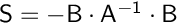 This is a square matrix. The cost to build exactly this matrix is prohibitive. Thus, one needs an approximation denoted by
An approximation of the Schur complement is needed by the following strategies:
"fgmres" (only with PETSc), "gcr" or "minres""uzawa_cg"The efficiency of the strategy to solve the saddle-point problem is related to the quality of the approximation. Several types of approximation of the Schur complement are available and a synthesis of the different options is gathered in the following table.
| key value | description | related type | family |
|---|---|---|---|
"none" | No approximation. The Schur complement approximation is not used. | CS_PARAM_SADDLE_SCHUR_NONE | all |
"diag_inv" | 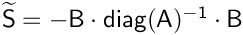 | CS_PARAM_SADDLE_SCHUR_DIAG_INVERSE | saturne, petsc |
"identity" | The identity matrix is used. | CS_PARAM_SADDLE_SCHUR_IDENTITY | saturne, petsc |
"lumped_inv" | 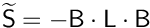 where where  , ,  is the vector fill with the value 1. is the vector fill with the value 1. | CS_PARAM_SADDLE_SCHUR_LUMPED_INVERSE | saturne |
"mass_scaled" | The pressure mass matrix is used with a scaling coefficient. This scaling coefficient is related to the viscosity for instance when dealing with the Navier-Stokes system. | CS_PARAM_SADDLE_SCHUR_MASS_SCALED | saturne |
"mass_scaled_diag_inv" | This is a combination of the "mass_scaled" and "diag_inv" approximation. | CS_PARAM_SADDLE_SCHUR_MASS_SCALED_DIAG_INVERSE | saturne |
"mass_scaled_lumped_inv" | This is a combination of the "mass_scaled" and "lumped_inv" approximation. | CS_PARAM_SADDLE_SCHUR_MASS_SCALED_LUMPED_INVERSE | saturne |
To set the way to approximate the Schur complement use
For the Schur approximation implying the "diag_inv" or the "lumped_inv" approximation, one needs to build and then solve a linear system associated to the Schur approximation. In the case of the "lumped_inv", an additionnal linear system is solved to define the vector  from the resolution of
  . Please consider the examples below for more details.
In the first example, one assumes that the saddle-point solver is associated to the structure \cs_equation_param_t nammed mom_eqp. For instance, one uses a gcr strategy for solving the saddle-point problem. This is one of the simpliest settings for the Schur complement approximation. The "mass_scaled" approximation is well-suited for solving the Stokes problem since the pressure mass matrix is a rather good approximation (in terms of spectral behavior) of the Schur complement.
In the second example, one assumes that the saddle-point solver is associated to the structure \cs_equation_param_t nammed mom_eqp. One now considers a more elaborated approximation which needs to solve a system implying the Schur complement approximation.
In the third and last example, one assumes that the saddle-point solver is associated to the structure \cs_equation_param_t nammed mom_eqp. One now considers a more elaborated approximation which needs to solve a system implying the Schur complement approximation and an additional system to build the Schur complement approximation (the system related to ).
In some cases, the initial residual is very small leading to an immediate exit. If this happens and it should not be the case, one can specify a stronger criterion to trigger the immediate exit. In the function cs_user_linear_solvers, add the following lines for instance:
An immediate exit is possible (i.e. there is no solve) when the norm of the right-hand side is equal to zero or very close to zero (cs_sles_set_epzero). To allow this kind of behavior for the SLES associated to an equation, one has to set the key CS_EQKEY_SOLVER_NO_OP to true.