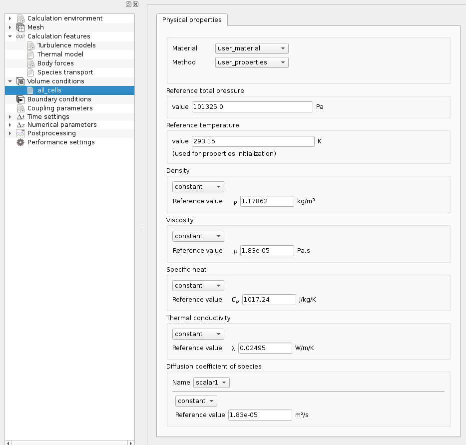
Basic variable physical properties

When the fluid properties are not constant, the user may define the variation laws in the GUI or in the cs_user_physical_properties user-defined function, which is called at each time step. In the GUI, in the item Fluid properties under the Physical properties section , the variation laws are defined for the fluid density, viscosity, specific heat, thermal conductivity and scalar dynamic dynamic diffusivity as shown on the figures below.

Physical properties - Fluid properties

Variable (in space and time) properties can be defined using a formula editor, described in a later section.

The validity of the variation laws is the user's responsibility, and should be verified, particularly when non-linear laws are defined (for instance, a third-degree polynomial law may produce negative density values).

Warning

If the user wishes to impose a variable density or viscosity in cs_user_physical_properties, a variable or viscosity must first be selected in the GUI, or irovar or ivivar respectively must have been set to 1 in cs_glob_fluid_properties at an earlier stage (i.e. in cs_user_parameters).
In order to impose a physical property (ρ, μ, λ C_p), a reference value should be provided (except possibly for some physical models in which this is predefined.
By default, the C_p coefficient and the dynamic diffusivity for the scalars (conductivity λ for the temperature) are considered as constant in time and uniform in space, with the cp0 and the value associated to the field's diffusivity_ref keyword. To assign a variable value to C_p, the user must specify it in the GUI (with a user law) or set icp to 1 for cs_glob_fluid_properties in cs_user_parameters.c, and assign a value for each cell to the array cpro_cp which can be accessed through ->val.
In the same manner, to have a variable dynamic diffusivity for a given scalar}, the user must specify it in the GUI (with a user law) or set that field's diffusivity_id keyword to a value > -1 in cs_user_parameters.c before assigning values to the matching field.
For variable (in space) properties, it is always possible to assign a value in the GUI and overwrite it in cs_user_physical_properties.
The scalar diffusivity_id must not be defined for user scalars representing the average of the square of the fluctuations of another scalar, because the diffusivity of a user scalar representing the average of the square of the fluctuations of another scalar is based on the diffusivity of this parent scalar.

Using physical property libraries

CoolProp

When code_saturne has been built with CoolProp support, that library may be used to compute fluid properties selected directly from the GUI.

Note than when properties are variable, CoolProp will default to using tabulated data properties for better performance. The choice of the backend may otherwise be forced by calling cs_physical_properties_set_coolprop_backend from the cs_user_model user-defined function.

Note that when using tables, CoolProp stores tabulations in the $HOME/.CoolProp/Tables directory by default, though this can be modified by defining the ALTERNATIVE_TABLES_DIRECTORY environment variable. Each table requires about 20 Mb in size, and will be created the first time a given fluid is used in a computation. The initialization time for that run will reflect this, though subsequent runs will simply read the data. Tabulation data may be cleaned by removing or cleaning this directory, and its size may otherwise be limited by using the MAXIMUM_TABLE_DIRECTORY_SIZE_IN_GB environment variable.

Turbulence model properties

Modification of the turbulent viscosity

The usvist user-defined subroutine can be used to modify the calculation of the turbulent viscosity, i.e. μ_t in $kg.m^{-1}.s^{-1}$ . The correspondig field, turbulent_viscosity, can be accessed by calling field_get_val_s(ivisct, cpro_visct). The subroutine is called at the beginning of every time step, after the calculation of the physical parameters of the flow and of the "conventional" value of μ_t corresponding to the chosen turbulence model.

Warning: The calculation of the turbulent viscosity being a particularly sensitive aspect, bad choices here may seriously distort the results.

Modification of the variable C of the dynamic LES model

The cs_user_physical_properties_smagorinsky_c user-defined function can be used to modify the calculation of the variable C of the LES sub-grid scale dynamic model.

It worth recalling that the LES approach introduces the notion of filtering between large eddies and small motions. The solved variables are said to be filtered in an "implicit" way. Sub-grid scale models ("dynamic" models) introduce in addition an explicit filtering.

The notations used for the definition of the variable C used in the dynamic models of code_saturne are specified below. These notations are the ones assumed in the document [3].

The value of a filtered by the explicit filter (of width $\widetilde{\overline{\Delta}}$ ) is called $\widetilde{a}$ and the value of a filtered by the implicit filter (of width $\overline{\Delta}$ ) is called $\overline{a}$ . We define:

$\begin{array}{ll} \overline{S}_{ij}=\frac{1}{2}(\frac{\partial \overline{u}_i}{\partial x_j} +\frac{\partial \overline{u}_j}{\partial x_i}) & ||\overline{S}||=\sqrt{2 \overline{S}_{ij}\overline{S}_{ij}}\\ \alpha_{ij}=-2\widetilde{\overline{\Delta}}^2 ||\widetilde{\overline{S}}|| \widetilde{\overline{S}}_{ij}& \beta_{ij}=-2\overline{\Delta}^2 ||\overline{S}|| \overline{S}_{ij}\\ L_{ij}=\widetilde{\overline{u}_i\overline{u}_j}- \widetilde{\overline{u}}_i\widetilde{\overline{u}}_j& M_{ij}=\alpha_{ij}-\widetilde{\beta}_{ij}\\ \end{array}$

In the framework of LES, the total viscosity (molecular + sub-grid) in $kg.m^{-1}.s^{-1}$ may be written in \CS:

$\begin{array}{llll} \mu_{\text{total}}&=&\mu+\mu_{\text{sub-grid}} & \text{\ \ if\ \ }\mu_{\text{sub-grid}}>0\\ &=&\mu & \text{\ \ otherwise }\\ \text{with\ }\mu_{\text{sub-grid}}&=&\rho C \overline{\Delta}^2 ||\overline{S}|| \end{array}$

$\overline{\Delta}$ is the width of the implicit filter, defined at the cell $\Omega_i$ by
$\overline{\Delta}=XLESFL*(ALES*|\Omega_i|)^{BLES}$

In the case of the Smagorinsky model, C is a constant which is worth . is the so-called Smagorinsky constant and is stored in the variable cs_turb_csmago.

In the case of the dynamic model, C is variable in time and in space. It is determined by $\displaystyle C=\frac{M_{ij}L{ij}}{M_{kl}M_{kl}}$ .

In practice, in order to increase the stability, the code does not use the value of C obtained in each cell, but an average with the values obtained in the neighboring cells (this average uses the extended neighborhood or other vertex neighbors and corresponds to the explicit filter). By default, the value calculated by the code is

$C=\frac{\widetilde{M_{ij}L{ij}}}{\widetilde{M_{kl}M_{kl}}}$

The cs_user_physical_properties_smagorinsky_c function (called at each time step, only when this model is active) allows to modify this value. It is for example possible to compute the local average after having computed the

$C=\widetilde{\left[\frac{M_{ij}L{ij}}{M_{kl}M_{kl}}\right]}$