|
8.2
general documentation
|


|
|
8.2
general documentation
|
|
When using the atmospheric module, a file called meteo may be added to a case's DATA directorys in order to provide vertical profiles of the main variables.
An atmospheric mesh has the following specific features:
 \upshape z = 1 m) near the ground to a few hundreds of meters at the top.
 and
and  .
.A topography map can be used to generate a mesh. In this case, the preprocessor mode is particularly useful to check the quality of the mesh (run type Mesh quality criteria).
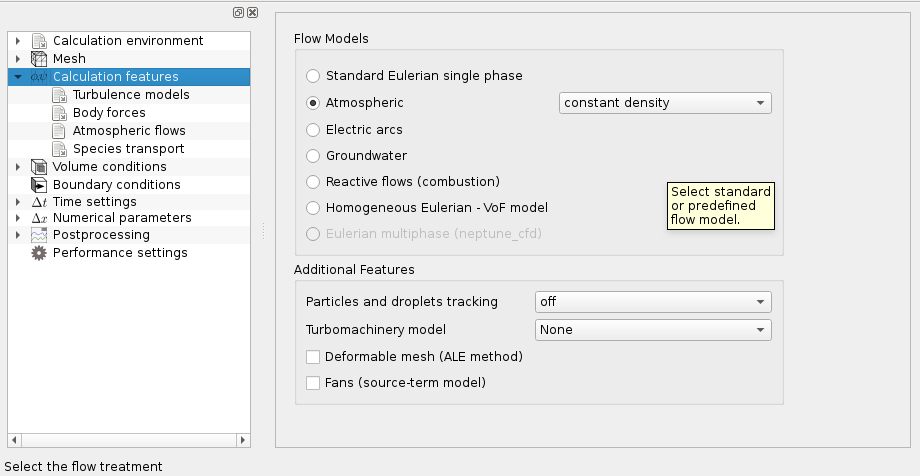
The GUI may be used to enable the atmospheric flow module and set up the following calculation parameters in the Thermophysical models - Calculation features page see fig:steady.
The user can choose one of the following atmospheric flow models:

 (
(  ), otherwise pressure and density won't be correctly computed.
 ( ), even if the density is constant.
The specific heat value has to be set to the atmospheric value  .
.
| Parameters | Constant density | Dry atmosphere | Humid atmosphere | Explanation |
|---|---|---|---|---|
| pressure boundary condition | Neumann first order | Extrapolation | Extrapolation | In case of Extrapolaion, the pressure gradient is assumed (and set) constant, whereas in case of Neumann first order, the pressure gradient is assumed (and set) to zero. |
| Improved pressure | no | yes | yes | If yes, exact balance between the hydrostatic part of the pressure gradient and the gravity term  g is numerically ensured. g is numerically ensured. |
| Gravity (gravity is assumed aligned with the z-axis) |  or (the latter is useful for scalar with drift) or (the latter is useful for scalar with drift) | | | |
| Thermal variable | no | potential temperature | liquid potential temperature | |
| Others variables | no | no | total water content, droplets number |
The meteo file can be used to define initial conditions for the different fields and to set up the inlet boundary conditions. For the velocity field, code_saturne can automatically detect if the boundary is an inlet boundary or an outflow boundary, according to the wind speed components given in the meteo file with respect to the boundary face orientation. This is often used for the lateral boundaries of the atmospheric domain, especially if the profile is evolving in time. In the case of inlet flow, the data given in the meteo file will be used as the input data (Dirichlet boundary condition) for velocity, temperature, humidity and turbulent variables. In the case of outflow, a Neumann boundary condition is automatically imposed (except for the pressure). The unit of temperature in the meteo file is the degree Celsius whereas the unit in the GUI is the kelvin.
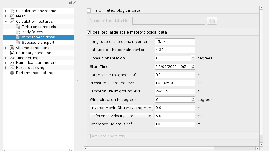
To be taken into account, the meteo file has to be selected in the GUI (Atmospheric flows page, see fig:meteo) and the check box on the side ticked. This file gives the profiles of prognostic atmospheric variables containing one or a list of time stamps. The file has to be put in the DATA directory.
An example of file meteo is given in the directory data/user/meteo. The file format has to be strictly respected. The horizontal coordinates are not used at the present time (except when boundary conditions are based on several meteorological vertical profiles) and the vertical profiles are defined with the altitude above sea level. The highest altitude of the profile should be above the top of the simulation domain and the lowest altitude of the profile should be below or equal to the lowest level of the simulation domain. The line at the end of the meteo file should not be empty.
If the boundary conditions are variable in time, the vertical profiles for the different time stamps have to be written sequentially in the meteo file.
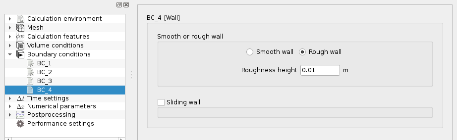
You can also set the profiles of atmospheric variables directly in the GUI. The following boundary conditions can be selected in the GUI:


In some cases, especially when outputs of a mesoscale model are used, you need to build input boundary conditions from several meteorological vertical wind profiles. Cressman interpolation is then used to create the boundary conditions. The following files need to be put in the \texttt{DATA} directory: \item All meteo files giving the different vertical profiles of prognostic variables (wind, temperature, turbulent kinetic energy and dissipation).
The following files should be put in the SRC directory:
User-defined functions may be used when the graphical user interface is not sufficient to set up the calculation. We provide some examples of user file for atmospheric application:
To simulate the atmospheric dispersion of pollutant, one first need to define the source(s) term(s). That is to say the location i.e. the list of cells or boundary faces, the total air flow, the emitted mass fraction of pollutant, the emission temperature and the speed with the associated turbulent parameters. The mass fraction of pollutant is simulated through a user added scalar that could be a scalar with drift if wanted (aerosols for example).
The simulations can be done using 2 different methods:
With the first method, the same problem of sources interactions appears, and moreover standard Dirichlet conditions should not be used (use itypfb=i_convective_inlet and icodcl=13 instead) as the exact emission rate cannot be prescribed because the diffusive part (usually negligible) cannot be quantified. Additionally, it requires that the boundary faces of the emission are explicitly represented in the mesh.
Finally the second method does not take into account the jet effect of the emission and so must be used only if it is sure that the emission does not modify the flow.
Whatever solution is chosen, the mass conservation should be verified by using for example the cs_user_extra_operations-scalar_balance.c file.
This model is based on the force restore model ([9]). It takes into account heat and humidity exchanges between the ground and the atmosphere at daily scale and the time evolution of ground surface temperature and humidity. Surface temperature is calculated with a prognostic equation whereas a 2-layers model is used to compute surface humidity.
The parameter iatsoil in the file atini0.f90 needs to be equal to one to activate the model. Then, the source file solvar.f90 is used.
Three variables need to be initialized in the file atini0.f90: deep soil temperature, surface temperature and humidity.
The user needs to give the values of the model constants in the file solcat.f90: roughness length, albedo, emissivity...
In case of a 3D simulation domain, land use data has to be provided for the domain. Values of model constants for the land use categories have also to be provided.
The 1D-radiative model calculates the radiative exchange between different atmospheric layers and the surface radiative fluxes.
The radiative exchange is computed separately for two wave lengths intervals
This 1D-radiative model is needed if the soil/atmosphere interaction model is activated.
This model is activated if the parameter iatra1 is equal to one in the file cs_users_parameters.f90.
For more details on the topic of atmospheric boundary layers, see [18].
![\[ \theta =T\left(\frac{P}{P_{r}}\right)^{-\frac{R_{d}}{C_{p}}} \]](form_832.png)
![\[ \theta_{l} = \theta \left( 1-\frac{L}{C_{p}T} q_{l} \right) \]](form_833.png)
![\[ T_{v} = \left(1+0.61q\right)T \]](form_834.png)
![\[ P = \rho \frac{R}{M_{d}}\left(1+0,61q\right)T \]](form_835.png)
 .
.
![\[ \frac{\partial P}{\partial z} = -\rho g \]](form_837.png)
| Constant name | Symbol | Values | Unit |
|---|---|---|---|
| Gravity acceleration at sea level |  |  |  |
| Effective Molecular Mass for dry air |  |  |  |
| Standard reference pressure |  |  |  |
| Universal gas constant |  |  |  |
| Gas constant for dry air |  |  |  |
| Variable name | Symbol |
|---|---|
| Specific heat capacity of dry air |  |
| Atmospheric pressure |  |
| Specific humidity |  |
| Specific content for liquid water |  |
| Temperature |  |
| Virtual temperature |  |
| Potential temperature |  |
| Liquid potential temperature |  |
| Latent heat of vaporization |  |
| Density |  |
| Altitude |  |
This part is a list of recommendations for atmospheric numerical simulations.
 ).
).In some cases, results can be improved with the following modifications:
 model in stable atmospheric condition). In those cases, it is suggested to put an artificial molecular viscosity around
  .
. or/and
  ).
).