Minimalist example to solve a Laplacian using CDO schemes

Table of Contents

• Introduction
• First step: Preprocessing
• Second step: Activate CDO and add a user-defined equation
• Third step: Define the equation to solve
• Last step: Run the computation
• To go beyond

Introduction

Here is a minimalist example to solve a scalar-valued Laplacian problem (an isotropic diffusion equation). Since one considers the CDO framework to solve this problem, this enables a quick start with this framework. This simple example is performed in three steps:

• Define a mesh and its boundary zones (done in the GUI)
• Activate the CDO and create the equation to solve (done in the function cs_user_model of the user source file cs_user_parameters.c)
• Define the equation to solve and set the boundary conditions (done in the function cs_user_finalize_setup of the user source file cs_user_parameters.c)

For a very beginner, one strongly advises to read the page Case directory structure.

In a terminal, write the following syntax for the creation of a new study with a new case:

code_saturne create --study STUDY CASE_NAME1

which creates a study directory STUDY with case sub-directory CASE_NAME1. If no case name is given, a default case directory called CASE1 is created.

First step: Preprocessing

One assumes that the mesh is a Cartesian mesh generated using the GUI but other ways are also possible. A more detail description of the different preprocessing possibilities is available here

GUI: Cartesian mesh definition

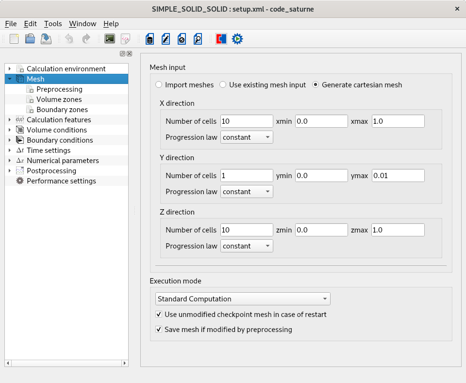
The generated Cartesian is built with 6 mesh face groups collecting boundary faces and named X0, X1, Y0, Y1, Z0 and Z1. These mesh face groups are used to define the two boundary zones needed for this example. One proceeds as detailed in the GUI screenshot.

Second step: Activate CDO and add a user-defined equation

The second step corresponds to the edition of the user source file named cs_user_parameters.c and especially the function cs_user_model

Click on the icon displayed just below in the GUI toolbar which corresponds to "Open the source file editor"

Then right-click on the file named REFERENCE/cs_user_parameters.c and select Copy to SRC. Then, you can choose your favorite file editor to add in the function cs_user_model the following lines.

  {
    /* Activate CDO/HHO mode */
 
    cs_param_cdo_mode_set(CS_PARAM_CDO_MODE_ONLY);
 
    /* Add a user-defined equation */
 
    cs_equation_add_user("Laplacian", /* equation name */
                         "potential", /* associated variable field name */
                         1,           /* dimension of the unknown */
                      CS_PARAM_BC_HMG_NEUMANN); /* default boundary condition */
  }

This first activates the CDO module (please refer to Activation of CDO/HHO schemes for more details) and then add a new scalar equation called Laplacian with an unknown named potential. This will be the name of the associated variable field. A default boundary condition is also defined and it corresponds to an homogeneous Neumann boundary condition. If no other boundary condition is defined, then all the boundary faces will be associated to this default definition.

Third step: Define the equation to solve

The last step corresponds to the modification of the function cs_user_finalize_setup in the file cs_user_parameters.c

  {
    cs_equation_param_t  *eqp = cs_equation_param_by_name("Laplacian");
 
    /* The property named "unity" is defined by default. Associate this
       property to the diffusion term and add it to the equation settings. */
 
    cs_equation_add_diffusion(eqp, cs_property_by_name("unity"));
 
    /* Boundary conditions (One assumes that two boundary zones named "X0" and
       "X1" exist. This is the case for instance if a Cartesian mesh is
       generated from the GUI. The two boundary zones are added in the
       GUI. Label is set to "X0" (resp. "X1") and selection criterion "X0"
       (resp. "X1").
    */
 
    cs_real_t  T0 = 0, T1 = 1;
    cs_equation_add_bc_by_value(eqp, CS_PARAM_BC_DIRICHLET, "X0", &T0);
    cs_equation_add_bc_by_value(eqp, CS_PARAM_BC_DIRICHLET, "X1", &T1);
  }

After having retrieved the structure cs_equation_param_t associated to the equation to solve, one first add a diffusion term which is associated to the default property named unity. Then, one defines two Dirichlet boundary conditions: a first one on the left side (X0) with a value equal to 0 and a second one on the right side (X1) with a value equal to 1.

Last step: Run the computation

For a very beginner, one strongly advises to read the page Running a calculation.

In a terminal, write the following syntax when your current directory corresponds to one of the sub-directories of a case.

code_saturne run

To go beyond

In order to change the numerical settings related to an equation call the function cs_equation_param_set inside the user function named cs_user_parameters in the file cs_user_parameters.c

Here are some examples of numerical settings:

  {
    cs_equation_param_t  *eqp = cs_equation_param_by_name("AdvDiff.Upw");
 
    /* The modification of the space discretization should be apply first */
    cs_equation_param_set(eqp, CS_EQKEY_SPACE_SCHEME, "cdo_vb");
    cs_equation_param_set(eqp, CS_EQKEY_ADV_SCHEME, "upwind");
 
    /* Modify other parameters than the space discretization */
    cs_equation_param_set(eqp, CS_EQKEY_VERBOSITY, "2");
    cs_equation_param_set(eqp, CS_EQKEY_HODGE_DIFF_ALGO, "cost");
    cs_equation_param_set(eqp, CS_EQKEY_HODGE_DIFF_COEF, "dga");
 
    /* Linear algebra settings */
#if defined(HAVE_PETSC)
    cs_equation_param_set(eqp, CS_EQKEY_SOLVER_FAMILY, "petsc");
    cs_equation_param_set(eqp, CS_EQKEY_ITSOL, "cg");
    cs_equation_param_set(eqp, CS_EQKEY_PRECOND, "amg");
#else
    cs_equation_param_set(eqp, CS_EQKEY_SOLVER_FAMILY, "cs");
    cs_equation_param_set(eqp, CS_EQKEY_PRECOND, "jacobi");
    cs_equation_param_set(eqp, CS_EQKEY_ITSOL, "cg");
#endif
    cs_equation_param_set(eqp, CS_EQKEY_ITSOL_MAX_ITER, "2500");
    cs_equation_param_set(eqp, CS_EQKEY_ITSOL_RTOL, "1e-12");
    cs_equation_param_set(eqp, CS_EQKEY_ITSOL_RESNORM_TYPE, "false");
 
  }

This relies on a key value principle. The available keys are listed here

For the reader willing to get a better understanding of the mathematical concepts underpinning the CDO schemes, one refers to the PhD thesis entitled Compatible Discrete Operator schemes on polyhedral meshes for elliptic and Stokes equations [3]