General information

The particle-tracking (or Lagrangian) module enables the simulation of poly-dispersed particulate flows, by calculating the trajectories of individual particles, mainly characterized by their diameter and density (if no heat nor mass transfer between particle and fluid are activated).
The standard use of the particle-tracking module follows the Moments/PDF approach: the instantaneous properties of the underlying flow needed to calculate the particle motion are reconstructed from the averaged values (obtained by Reynolds-Averaged Navier-Stokes simulation) by using stochastic processes. The statistics of interest are then obtained through Monte-Carlo simulation.
As a consequence, is is important to emphasize that the most important (and physically meaningful) results of a particle-tracking calculation following the Moments/PDF approach are statistics. Volume and surface statistics, steady or unsteady, can be calculated. Individual particle trajectories (as 1D, EnSight-readable cases) and displacements (as EnSight-readable animations) can also be provided, but only for illustrative purposes.

Activating the particle-tracking module

The activation of the particle-tracking module is performed either:

in the Graphical User Interface (GUI): Calculation features --> Homogeneous Eulerian - VoF model --> particles and droplets tracking
or in the user function cs_user_lagr_model.

Basic guidelines for standard simulations

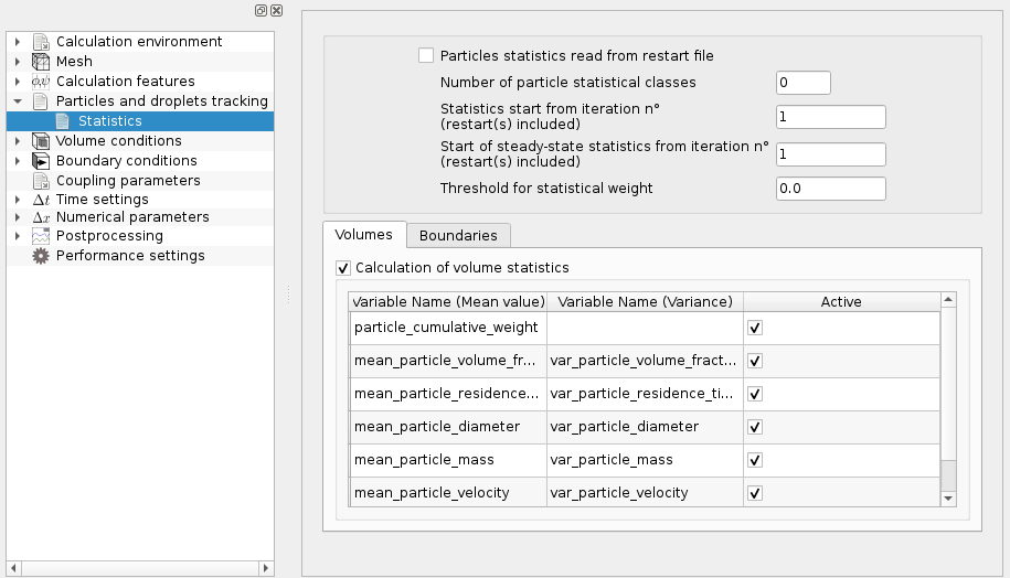
Except for cases in which the flow conditions depend on time, it is generally recommended to perform a first Lagrangian calculation whose aim is to reach a steady-state (i.e. to reach a time starting from which the relevant statistics do not depend on time anymore). In a second step, a calculation restart is done to calculate the statistics. When the single-phase flow is steady and the particle volume fraction is low enough to neglect the particles influence on the continuous phase behaviour, it is recommended to perform a Lagrangian calculation on a frozen field.

It is then possible to calculate steady-state volumetric statistics and to give a statistical weight higher than 1 to the particles, in order to reduce the number of simulated (numerical) particles to treat while keeping the right concentrations. Otherwise, when the continuous phase flow is steady, but the two-coupling coupling must be taken into consideration, it is still possible to activate steady statistics. When the continuous phase flow is unsteady, it is no longer possible to use steady statistics. To have correct statistics at every moment in the whole calculation domain, it is imperative to have an established particle seeding and it is recommended (when it is possible) not to impose statistical weights different from the unity.

Finally, when the so-called complete model is used for turbulent dispersion modelling, the user must make sure that the volumetric statistics are directly used for the calculation of the locally undisturbed fluid flow field.

When the thermal evolution of the particles is activated, the associated particulate scalars are always the inclusion temperature and the locally undisturbed fluid flow temperature expressed in degrees Celsius, whatever the thermal scalar associated with the continuous phase is (i.e. temperature or enthalpy). If the thermal scalar associated with the continuous phase is the temperature in Kelvin, the unit is converted automatically into Celsius. If the thermal scalar associated with the continuous phase is the enthalpy, a temperature property or postprocessing field must be defined. In all cases, the thermal backward coupling of the dispersed phase on the continuous phase is adapted to the thermal scalar transported by the fluid.

Prescribing the main modelling parameters

Use of the GUI

In the GUI, the selection of the Lagrangian module activates the heading Particle and droplets tracking in the tree menu. The initialization is performed in the three items included in this heading:

Global settings. The user defines in this item the kind of Euler/Lagrange multi-phase treatment, the main parameters, and the specific physics associated with the particles, see Figure 1
Statistics. The user can select the volume and boundary statistics to be post-processed see Figure 2.
Output. An additional entry in the postprocessing section allows defining the output frequency and post-processing options for particles and selecting the variables that will appear in the log see Figure 3.

Lagrangian module - View of the _Global Settings_ page

Lagrangian module - statistics

Lagrangian module - output

Use of the function cs_user_lagr_model

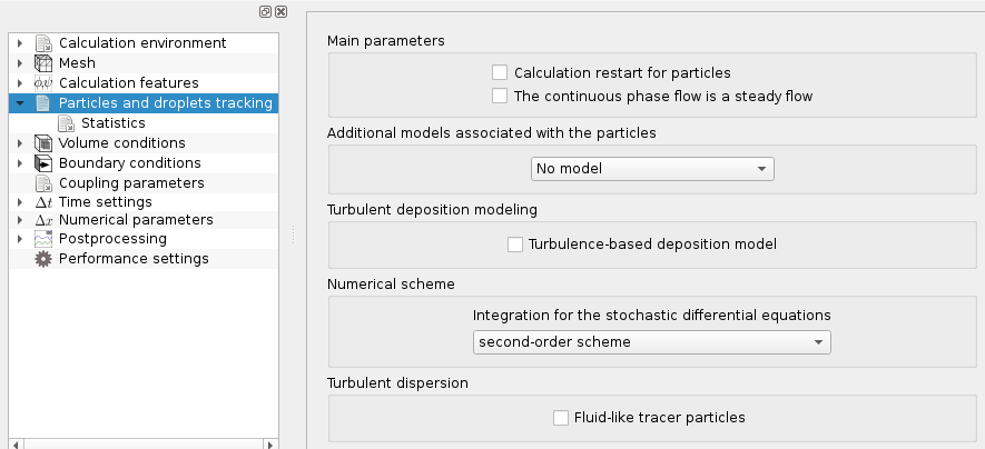
When the GUI is not used, cs_user_lagr_model must be completed. This function gathers in different headings all the keywords which are necessary to configure the Lagrangian module. The different headings refer to:

the global configuration parameters
the specific physical models describing the particle behaviour
the backward coupling (influence of the dispersed phase on the continuous phase)
the numerical parameters
the volumetric statistics
the boundary statistics

For more details about the different parameters and some examples, the user may refer to examples

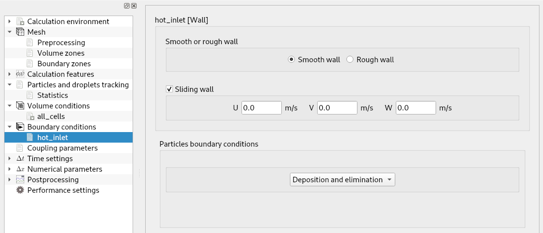
Prescribing particle boundary conditions

In the framework of the multiphase Lagrangian modelling, the management of the boundary conditions concerns the particle behaviour when there is an interaction between its trajectory and a boundary face. These boundary conditions may be imposed independently of those concerning the Eulerian fluid phase (but they are of course generally consistent). The boundary condition zones are actually redefined by the Lagrangian module (boundary zones), and a type of particle behaviour is associated with each one. The boundary conditions related to particles can be defined in the Graphical User Interface (GUI) or in the cs_user_lagr_boundary_conditions.c} file. More advanced user-defined boundary conditions can be prescribed in the cs_user_lagr_in function from cs_user_lagr_particle.c}.

Use of the GUI

In the GUI, selecting the Lagrangian module in the activates the item Particle boundary conditions under the heading Boundary conditions in the tree menu. Different options are available depending on the type of standard boundary conditions selected (wall, inlet/outlet, etc...), see Figure 3.

Lagrangian module - boundary conditions

Advanced particle-tracking set-up

In this section, some information is provided for a more advanced numerical set-up of a particle-tracking simulation.

User-defined stochastic differential equations

An adaptation in the cs_user_lagr_sde function is required if supplementary user variables are added to the particle state vector for more explanation see SDE within the Lagrangian model.

If necessary, the thermal characteristic time $\tau_c$ , whose calculation can be modified by the user in the function cs_user_lagr_rt.

User-defined particle relaxation time

The particle relaxation time may be modified in the cs_user_lagr_rt function according to the chosen formulation of the drag coefficient. The particle relaxation time, modified or not by the user, is available in the array taup see Calculation of the particle relaxation time for examples

User-defined particle thermal characteristic time

The particle thermal characteristic time may be modified in the cs_user_lagr_rt_t function according to the chosen correlation for the calculation of the Nusselt number see Computation of the thermal relaxation time of the particles for examples.