|
8.0
general documentation
|


|
|
8.0
general documentation
|
|
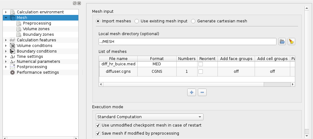
This page provides additional details on mesh import and preprocessing steps, as well as how mesh regions can be managed in the code_saturne Solver.
Referring to the modules described in the base architecture presentation, a mesh can be imported using the code_saturne Preprocessor, than further preprocessed in the Solver's initialization steps.
Importing meshes is done by the Preprocessor module, while most other preprocessing operations are done mainly by the code Solver (except for element orientation checking, which is done by the Preprocessor).
The Preprocessor module of code_saturne reads the mesh file(s) (under any supported format) and translates the necessary information into a Solver input file.
When multiple meshes are used, the Preprocessor is called once per mesh, and each resulting output is added in a mesh_input directory (instead of a single mesh_input.csm file).
Face and cell mesh-defined properties and selection
Throughout the use of code_saturne, including the selection of specific mesh sections for preprocessing operations, it is also useful to understand how high-level mesh element selection can be handled.
The code_saturne run operation automatically calls the Preprocessor for every mesh specified by the user with the GUI or in the MESHES list defined in cs_user_scripys.py:define_domain_parameters.
The executable of the Preprocessor module is named cs_preprocess, and is normally called through the run script, so it is not fount in the main executable program search paths.
Nonetheless, it may be useful to call the Preprocessor manually in certain situations, especially for frequent verification when building a mesh, so its use is described here. Verification may also be done using the GUI or the mesh quality check mode of the general run script.
The Preprocessor is controlled using command-line arguments. A few environment variables allow advanced users to modify its behavior or to obtain a trace of memory management. If needed, it can be called directly on most systems using the following syntax:
Note that on some systems (such as OpenSUSE), libexec may be replaced bylib`.
To obtain a description of all available option, type:
In the following sections, the ${install_prefix}/libexec/code_saturne prefix is omitted for conciseness. Main choices are done using command-line options. For example:
cs_preprocess --num 2 fluid.med
means that we read the second mesh defined in the fluid.med file, while:
cs_preprocess --no-write --post-volume med fluid.msh
means that we read file fluid.msh, and do not produce a mesh_input.csm file, but do output fluid.med file (effectively converting a Gmsh file to a MED file).
Any use of the Preprocessor requires one mesh file (except for cs_preprocess and cs_preprocess -h which respectively print the version number and list of options). This file is selected as the last argument to cs_preprocess, and its format is usually automatically determined based on its extension, but a --format option allows forcing the format choice of the selected file.
For formats allowing multiple meshes in a single file, the --num option followed by a strictly positive integer allows selection of a specific mesh; by default, the first mesh is selected.
For meshes in CGNS format, we may in addition use the --grp-cel or --grp-fac options, followed by the section or zone keywords, to define additional groups of cell or faces based on the organization of the mesh in sections or zones. These sub-options have no effect on meshes of other formats.
By default, the Preprocessor does not generate any post-processor output. By adding --post-volume [format], with the optional format argument being one of ensight, med, or cgns to the command-line arguments, the output of the volume mesh to the default or indicated format is provoked.
In case of errors, output of error visualization output is always produced, and by adding --post-error [format], the format of that output may be selected (from one of ensight, med, or cgns, assuming MED and CGNS are available),
Correction of element orientation is possible and can be activated using the --reorient option.
Note that we cannot guarantee correction (or even detection) of a bad orientation in all cases. Not all local numbering possibilities of elements are tested, as we focus on "common" numbering permutations. Moreover, the algorithms used may produce false positives or fail to find a correct renumbering in the case of highly non convex elements. In this case, nothing may be done short of modifying the mesh, as without a convexity hypothesis, it is not always possible to choose between two possible definitions starting from a point set.
With a post-processing option such as --post-error or, --post-volume, visualizable meshes of corrected elements as well as remaining badly oriented elements are generated.
Some functions of the Preprocessor are based on external libraries, which may not always be available. It is thus possible to configure and compile the Preprocessor so as not to use these libraries. When running the Preprocessor, the supported options are printed. The following optional libraries may be used:
.gz extension. This is limited to formats not already based on an external library (i.e. it is not usable with CGNS, MED, or CCM files), and has memory and CPU time overhead, but may be practical. Without this library, files must be uncompressed before use.Note that the Preprocessor is in general capable of reading all "classical" element types present in mesh files (triangles, quadrangles, tetrahedra, pyramids, prisms, and hexahedra). Quadratic or cubic elements are converted upon reading into their linear counterparts. Vertices referenced by no element (isolated vertices or centres of higher-degree elements) are discarded. Meshes are read in the order defined by the user and are appended, vertex and element indices being incremented appropriately. Entity labels (numbers) are not maintained, as they would probably not be unique when appending multiple meshes.
At this stage, volume elements are sorted by type, and the fluid domain post-processing output is generated if required.
In general, groups assigned to vertices are ignored. selections are thus based on faces or cells. with tools such as Simail, faces of volume elements may be referenced directly, while with I-deas or SALOME, a layer of surface elements bearing the required colors and groups must be added. Internally, the Preprocessor always considers that a layer of surface elements is added (i.e. when reading a Simail mesh, additional faces are generated to bear cell face colors. When building the  connectivity, all faces with the same topology are merged: the initial presence of two layers of identical surface elements belonging to different groups would thus lead to a calculation mesh with faces belonging to two groups).
Data passed to the Solver by the Preprocessor is transmitted using a binary file, using a big endian data representation, named mesh_input.csm (or contained in a mesh_input directory).
When using the Preprocessor for mesh verification, data for the Solver is not always needed. In this case, the --no-write option may avoid creating a Preprocessor output file.
 ,
,  , SSG, ...) used in code_saturne are "High-Reynolds" models. Therefore the size of the cells neighboring the wall must be greater than the thickness of the viscous sub-layer (at the wall,
  is required, and
  is preferable). If the mesh does not match this constraint, the results may be false (particularly if thermal phenomena are involved). For more details on these constraints, see the iturb keyword.
Conforming joining of possibly non-conforming meshes may be done by the solver, and defined either using the Graphical User Interface (GUI) or the cs_user_join user function. In the GUI, the user must add entries in the "Face joining" tab in the "Mesh/Proprocessing" page. The user may specify faces to be joined, and can also modify basic joining parameters.
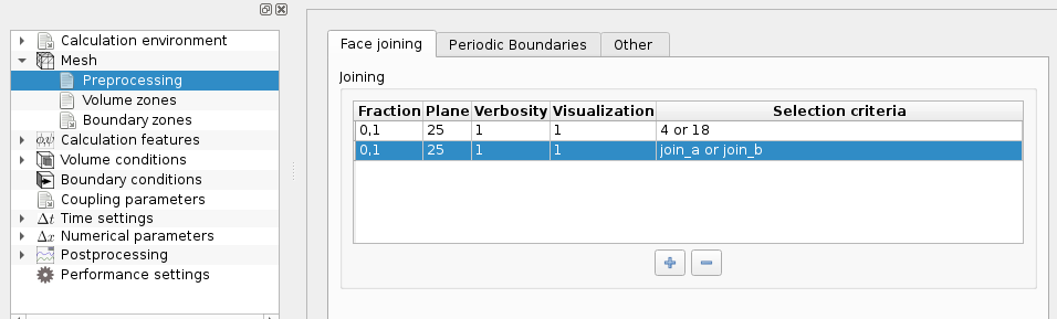
For a simple mesh, it is rarely useful to specify strict face selection criteria, as joining is sufficiently automated to detect which faces may actually be joined. For a more complex mesh, or a mesh with thin walls which we want to avoid transforming into interior faces, it is recommended to filter boundary faces that may be joined by using face selection criteria. This has the additional advantage of reducing the number of faces to test for in the intersection/overlap search, and thus improving the performance of the joining algorithm.
One may also modify tolerance criteria using 2 options, explained in the figure below:
fraction assigns value  (where
 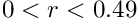 ) to the maximum intersection distance multiplier (
  by default). The maximum intersection distance for a given vertex is based on the length of the shortest incident edge, multiplied by r. The maximum intersection at a given point along an edge is interpolated from that at its vertices, as shown on the left of the figure
plane assigns the maximum angle between normals for two faces to be considered coplanar (  by default); this parameter is used in the second stage of the algorithm, to reconstruct conforming faces, as shown on the right of figure
As shown above, verbosity and visualization levels can also be set, to obtain more detailed logging of the joining operations, as well as detailed visualizable output of the selected and joined faces.
In practice, we are sometimes led to increase the maximum intersection distance multiplier to 0.2 or even 0.3 when joining curved surfaces, so that all intersection are detected. As this influences merging of vertices and thus simplification of reconstructed faces, but also deformation of "lateral" faces, it is recommended only to modify it if necessary. As for the plane parameter, its use has only been necessary on a few meshes up to now, to reduce the tolerance so that face reconstruction does not try to generate faces from initial faces on different surfaces.
This operation can be specified either using the GUI or the user-defined functions, as shown in various examples.
Advanced parameters may be set through user-defined functions by calling cs_join_set_advanced_param, as shown in the advanced mesh joining parameters examples section.
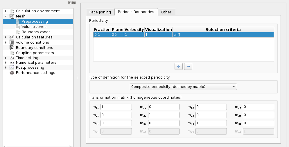
Handling of periodicity is based on an extension of conforming joining, as shown on the following figure. It is thus not necessary for the periodic faces to be conforming (though it usually leads to better mesh quality). All options relative to conforming joining of non-conforming faces also apply to periodicity. Note also that once pre-processed, 2 periodic faces have the same orientation (possibly adjusted by periodicity of rotation).
As with joining, it is recommended to filter boundary faces to process using a selection criterion. As many periodicities may be built as desired, as long as boundary faces are present. Once a periodicity is handled, faces having periodic matches do not appear as boundary faces, but as interior faces, and are thus not available anymore for other periodicities. Translation, rotation, and mixed periodicities can be defined.
This operation can be specified either using the GUI, as shown below, or by user-defined functions, as shown in various examples.
Quite a few other preprocessing operations are available in the Solver:
The cs_user_mesh_input function may be used for advanced modification of the main cs_mesh_t structure:
Examples with user-defined functions are provided in the mesh reading and modification examples subsection.
The cs_user_mesh_modify function may be used for advanced modification of the main cs_mesh_t structure.
The cs_user_mesh_modify function may be used for advanced modification of the main cs_mesh_t structure.
Examples with user-defined functions are provided in the general mesh modification examples subsection.
The principle of smoothers is to mitigate the local defects by averaging the mesh quality. This procedure may help for calculation robustness or/and results quality.
The cs_user_mesh_smoothe user function allows to apply smoothing operations.
An example with user-defined functions is provided in the mesh smoothing examples subsection.
The cs_mesh_smoother_unwarp function allows reducing face un-warping in the calculation mesh.
Be aware that, in some cases, this algorithm may degrade other mesh quality criteria.