Electric arcs module

The electric module is composed of a Joule effect module (CS JOULE EFFECT) and an electric arcs module (CS ELECTRIC ARCS).

The Joule effect module is designed to take into account that effect (for instance in glass furnaces) with real or complex potential in the enthalpy equation. The Laplace forces are not taken into account in the impulse momentum equation. Specific boundary conditions can be applied to account for the coupled effect of transformers (offset) in glass furnaces.

The electric arcs module is designed to take into account the Joule effect (only with real potential) in the enthalpy equation. The Laplace forces are taken into account in the impulse momentum equation.

Activating the electric arcs module

The electric arcs module is activated either:

• in the Graphical User Interface GUI: Calculation features --> Electrical arcs, the user can choose between Joule Effect for joule model and Joule Effect and Laplace Forces for electric arc
• or in the user function cs_user_model in cs_user_parameters.c file, by setting the cs_glob_physical_model_flag[CS_ELECTRIC_ARCS] or cs_glob_physical_model_flag[CS_JOULE_EFFECT] parameter to a non-null value.

Initialization of the variables

The function \re cs_user_initialization allows the user to initialize some of the specific physics variables prompted via cs_user_model. It is called only during the initialization of the calculation. As usual,the user has access to many geometric variables so that the zones can be treated separately if needed (see Electric arcs example).

The values of potential and its constituents are initialized if required.

It should be noted that the enthalpy is relevant.

• For the electric arcs module, the enthalpy value is taken from the temperature of reference t0 (given in cs_user_parameters.cpp) from the temperature-enthalpy tables supplied in the data file dp_ELE. The user must not intervene here.

For the Joule effect module, the value of enthalpy must be specified by the user. Examples of temperature to enthalpy conversion are given in cs_user_physical_properties.cpp). If not defined, a simple default law is used ( ).

Variable physical properties

All the laws of the variation of physical data of the fluid are written (when necessary) in the function cs_user_physical_properties.

Warning

For the electric module, it is here that all the physical variables are defined (including the relative cells and the eventual user scalars): cs_user_physical_properties is not used.

The user should ensure that the defined variation laws are valid for the whole range of variables. Particular care should be taken with non-linear laws (for example, a degree polynomial law giving negative values of density)

Warning

In the electric module, all of the physical properties are considered as variables and are therefore stored using the cs_field API. cp0, viscls0 and viscl0 are not used

For the Joule effect, the user is required to supply the physical properties in the function. Examples are given which are to be adapted by the user. If the temperature is to be determined to calculate the physical properties, the solved variable, enthalpy must be deduced. The preferred temperature-enthalpy law should be defined (a general example is provided in (cs_user_physical_properties), and can be used for the initialization of the variables in (cs_user_initialization)). For the electric arcs module, the physical properties are interpolated from the data file dp_ELE supplied by the user. Modifications are generally not necessary.

Boundary conditions

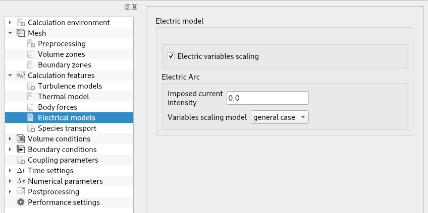
Boundary conditions can be handled in the GUI or in the cs_user_boundary_conditions function as usual (see Electric example. In the cs_user_boundary_conditions report, the main change from the users point of view concerns the specification of the boundary conditions of the potential, which isn't implied by default. The Dirichlet and Neumann conditions must be imposed explicitly using icodcl and rcodcl (as would be done for the classical scalar).

Furthermore, if one wishes to slow down the power dissipation (Joule effect module) or the current (electric arcs module) from the imposed values, they can be changed by the potential scalar as shown below:

• For the electric arcs, the imposed current intensity can be a fixed variable and initialize by the GUI see Figure 1

Imposed current intensity

• For the Joule model, the imposed power can be a fixed variable in the same way as the electric arcs.

Warning

In the case of alternating current, attention should be paid to the values of potential imposed at the limits: the variable named "real potential" represents an affective value if the current is in single phase, and a "real part" if not.

• For the Joule studies, a complex potential is sometimes needed (in the GUI Electrical model -> three-phase): this is the case in particular where the current has three phases. To have access to the phase of the potential, and not just to its amplitude.
• For the Joule studies in which one does not have access to the phases, the real potential (imaginary part =0) will suffice (in the GUI Electrical model -> AC/DC): this is obviously the case with continuous current, but also with single phase alternative current. In code_saturne there is only 1 variable for the potential, called "real potential". Pay attention to the fact that in alternate current, the "real potential" represents a effective value of potential, (in continuous current there is no such ambiguity).

Additions for transformers

The following additional boundary conditions must be defined for tansformers:

• the intensity at each electrode
• the voltage on each terminal of transformers. To achieve it, the intensity, the rvoltage at each termin, the Rvoltage, and the total intensity of the transformer are calculated.

Finally, a test is performed to check if the offset is zero or if a boundary face is in contact with the ground.