|
7.1
general documentation
|


|
|
7.1
general documentation
|
|
Logging and post-processing in code_saturne is handled so as to allow combining the ease of automatic outputs for the main variables and more advanced user-defined values or extracts.
Both the GUI and several functions present in cs_user_postprocess.c allow for managing post-processing output.
The main concepts are those of writers and meshes, which must be associated to produce outputs.
The combination of writers and meshes allows generating chronological outputs in EnSight, MED, or CGNS format, as well as in-situ visualization using ParaView Catalyst or ensemble data output to Melissa.
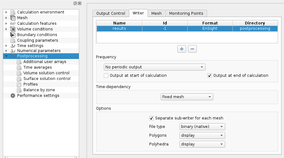
Using the GUI, writers can be managed and defined in the following page:
And postprocessing meshes can be handled in the following tab:
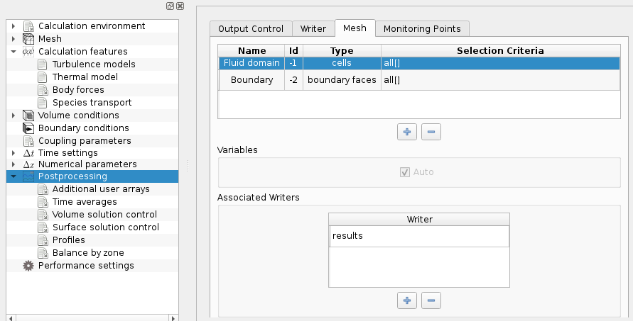
In order to allow the user to add an output format to the main output format, or to add a mesh to the default output, the lists of standard and user meshes and writers are not separated. Negative numbers are reserved for the non-user items. For instance, the mesh numbers -1 (CS_POST_MESH_VOLUME) and -2 (CS_POST_MESH_BOUNDARY) correspond respectively to the global mesh and to boundary faces, generated by default, and the writer -1 (CS_POST_WRITER_DEFAULT) corresponds to the default post-processing writer.
The user chooses the numbers corresponding to the post-processing meshes and writers he wants to create. These numbers must be positive integers. It is for example possible to associate a user mesh with the default post-processing writer (-1), or to add outputs regarding the boundary faces (-2) associated with a user writer.
For safety, the output frequency and the possibility to modify the post-processing meshes are associated with the writers rather than with the meshes. This logic avoids unwanted generation of inconsistent post-processing outputs. For instance, ParaView or EnSight would not be able to correctly read a case in which one field is output to a given part every 10 time steps, while another field is output to the same part every 200 time steps. If some fields should be output using different frequencies, using separate writers allow maintaining consistent output sets.
To prevent output related to a given mesh (including the default), the list of associated writers should be made empty.
Note that the default writer and meshes cannot be "undefined", though they may be renamed and their settings modified. A writer with no associated mesh is inactive, so removing the default writer from the list of writers associated to all meshes deactivates the default output.
Probe sets allow defining a number of probes at user-defined locations. The values of selected variables at these points may be output to specific writers, usually time plots (CSV or regular text files with one column per probe position and one line line output time step). These are typically used:
Profiles are defined as a special type of probe set, for which a curvilinear coordinate (the local profile coordinate) is defined, and are typically used not with time plots, but with simple plots (also in CSV or text format) where one file is associated to a single time step, and columns correspond to different variables, and lines to different positions along the profile.
Probe sets and profiles are defined as a special category of postp-rocessing meshes, so they can be also be used in combination with most other types of writers.
The GUI currently only allows handling a single (default) probe set for time plots. Probe coordinates can be entered directly or read from a CSV file.
Profiles are also handled in a specific manner, as they are automatically associated with default simple plot writers (CSV or text), and the associated variables may be selected specifically.
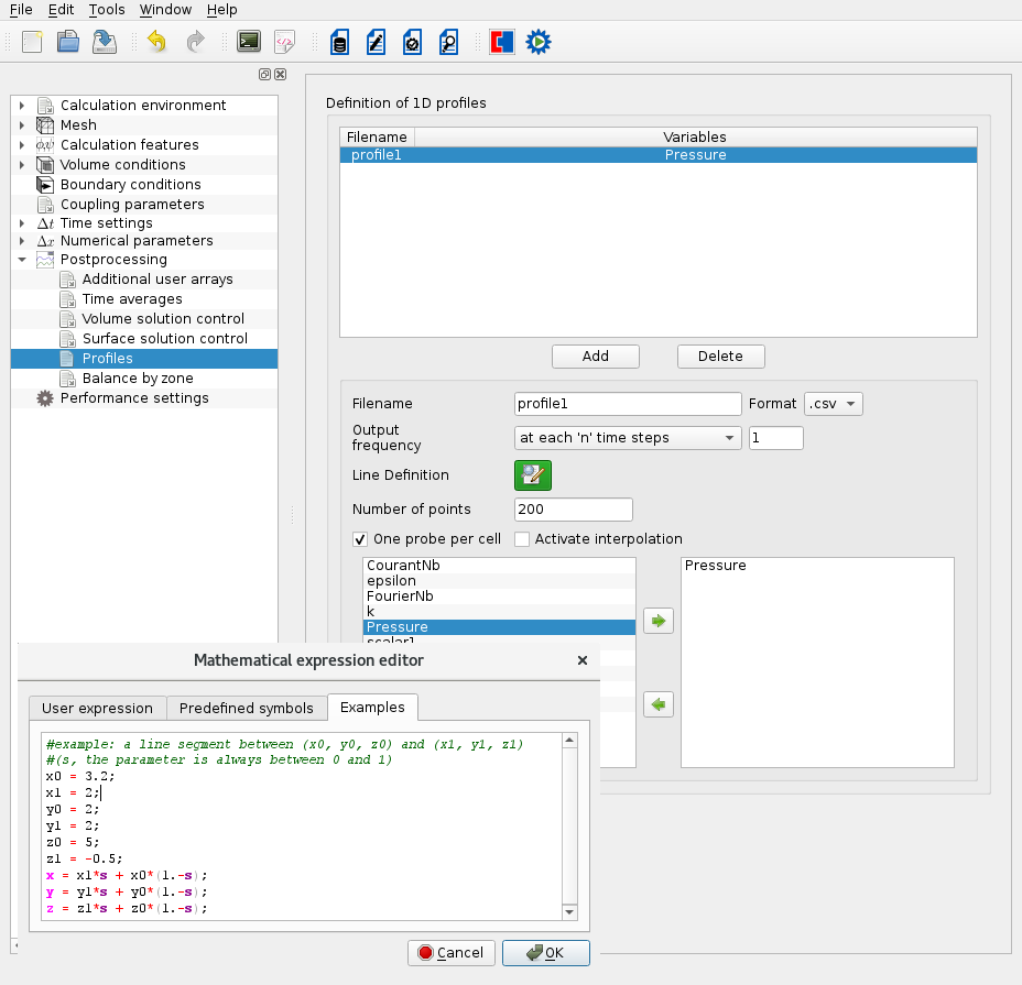
This presentation difference is mainly due to historic reasons (it predates the unification of probes, profiles, and other writers), not to a difference in the concepts used (so the logic may seem more consistent with user-defined functions).
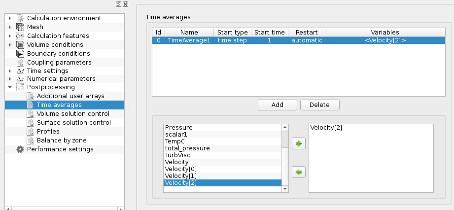
In code_saturne, it is possible to define time moments for existing variables (fields) or user-defined formulas, including both means and variances. This is limited to visualization output, so for example although the variance of a vector (which is a tensor due to the covariance terms) may be computed, the variance of a tensor may not (though that of specific components may always be computed).
This computation uses recurrence formulas, so at any given time steps, the mean or variance field values are always updated and accessible as a regular field. The computation of time moments may start at a user-defined time step of physical time so as not to include transient initialization data. In this case, the associated field values before actually starting the moment updates is 0.
Time moments may be defined in the GUI, as shown below, or using the cs_user_time_moments function in cs_user_parameters.c (see Time moment related options examples).
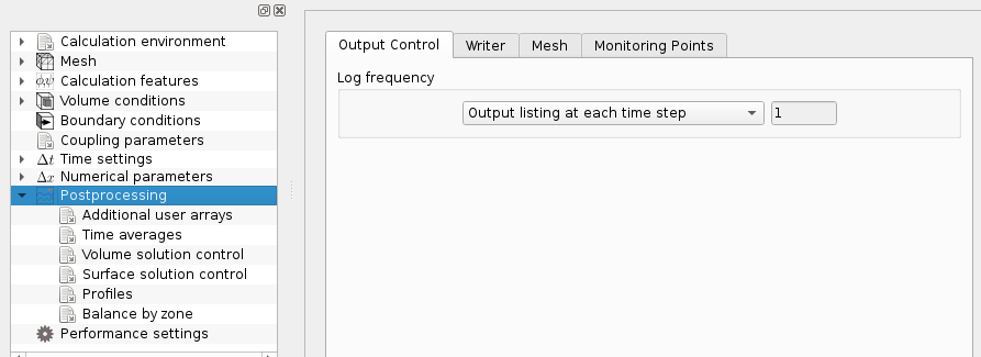
The logging output frequency may be managed using the GUI, as shown below. The first 10 time steps are always logged. When running many time steps, it recommended to use a logging period greater than 1 (20 or 100 are often sufficient), as logging each time step with even a moderate verbosity can lead to large run_solver.log files.
Note that logging verbosity is also influenced by the verbosity used for solved variables.
For the main computed values defined as fields, the GUI allows defining whether a given field with be associated using the default output meshes, the default probe set, and the main log.
This can also be handled using the post_vis and Output log field key values.
Also, the "auto variables" flag may be assigned to additional post-processing meshes so that output of fields behaves in a manner similar to that of the default post-processing mesh in the same category (for example the main volume mesh for a volume extract).
To output additional values, whether simply restricting output to a small subset of field or adding values based on specific computations or formulas, see the cs_user_postprocess_values user function and associated examples (in Definition of the variables to post-process).
Checking the convergence is difficult to automate, but code_saturne provides several tools to help manage this.
In the run_solver.log file for each run's output, a convergence section similar to the example below is available:
For each solved variable, it provides:
The time drift;
For a given variable  this is usually the following term:
![\[ \int_\Omega \left| \der{\varia}{t} \right|^2 \Delta t \dd \Omega / \int_\Omega \dd \Omega \]](form_854.png)
For the pressure variable it is computed in a different manner.
The time residual;
For a given variable this is the normalized L2 unsteady term:
![\[ \sqrt{\int_\Omega \left| \der{\varia}{t} \right|^2 \dd \Omega / \int_\Omega \left| \varia \right|^2 \dd \Omega} \]](form_733.png)
A file named residuals.csv is usually produced, containing the residuals for solved variables (as defined above), in an easy to plot CSV format.
It is recommended to place some probes at selected points of interest, so as to activate time plots of the main variable values at those points.
This allows both checking how values evolve over time in selected points and if that evolution is regular or "noisy".
 1.8.13